
10 Functional Programming 101
In this chapter, you will learn more about expressing complex logic in a functional language like Daml. Specifically, you’ll learn about
- Function signatures and functions
- Advanced control flow (
if...else, folds, recursion,when)
If you no longer have your chapter 7 and 8 projects set up, and want to look back at the code, please follow the setup instructions in 9 Working with Dependencies to get hold of the code for this chapter.
Note
There is a project template daml-intro-10 for this chapter, but it only contains a single source file with the code snippets embedded in this section.
The Haskell Connection
The previous chapters of this introduction to Daml have mostly covered the structure of templates, and their connection to the Daml Ledger Model. The logic of what happens within the do blocks of choices has been kept relatively simple. In this chapter, we will dive deeper into Daml’s expression language, the part that allows you to write logic inside those do blocks. But we can only scratch the surface here. Daml borrows a lot of its language from Haskell. If you want to dive deeper, or learn about specific aspects of the language you can refer to standard literature on Haskell. Some recommendations:
- Finding Success and Failure in Haskell (Julie Maronuki, Chris Martin)
- Haskell Programming from first principles (Christopher Allen, Julie Moronuki)
- Learn You a Haskell for Great Good! (Miran Lipovača)
- Programming in Haskell (Graham Hutton)
- Real World Haskell (Bryan O’Sullivan, Don Stewart, John Goerzen)
When comparing Daml to Haskell it’s worth noting:
- Haskell is a lazy language, which allows you to write things like
head [1..], meaning “take the first element of an infinite list”. Daml by contrast is strict. Expressions are fully evaluated, which means it is not possible to work with infinite data structures. - Daml has a
withsyntax for records, and dot syntax for record field access, neither of which present in Haskell. But Daml supports Haskell’s curly brace record notation. - Daml has a number of Haskell compiler extensions active by default.
- Daml doesn’t support all features of Haskell’s type system. For example, there are no existential types or GADTs.
- Actions are called Monads in Haskell.
Functions
In 3 Data types you learnt about one half of Daml’s type system: Data types. It’s now time to learn about the other, which are Function types. Function types in Daml can be spotted by looking for -> which can be read as “maps to”.
For example, the function signature Int -> Int maps an integer to another integer. There are many such functions, but one would be:
increment : Int -> Int
increment n = n + 1
You can see here that the function declaration and the function definitions are separate. The declaration can be omitted in cases where the type can be inferred by the compiler, but for top-level functions (ie ones at the same level as templates, directly under a module), it’s often a good idea to include them for readability.
In the case of increment it could have been omitted. Similarly, we could define a function add without a declaration:
add n m = n + m
If you do this, and wonder what type the compiler has inferred, you can hover over the function name in the IDE:
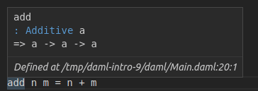
What you see here is a slightly more complex signature:
add : Additive a => a -> a -> a
There are two interesting things going on here:
- We have more than one
->. - We have a type parameter
awith a constraintAdditive a.
Function Application
Let’s start by looking at the right hand part a -> a -> a. The -> is right associative, meaning a -> a -> a is equivalent to a -> (a -> a). Using the “maps to” way of reading -> we get “a maps to a function that maps a to a”.
And this is indeed what happens. We can define a different version of increment by partially applying add:
increment2 = add 1
If you try this out in your IDE, you’ll see that the compiler infers type Int -> Int again. It can do so because of the literal 1 : Int.
So if we have a function f : a -> b -> c -> d and a value valA : a, we get f valA : b -> c -> d, ie we can apply the function argument by argument. If we also had valB : b, we would have f valA valB : c -> d. What this tells you is that function application is left associative: f valA valB == (f valA) valB.
Infix Functions
Now add is clearly just an alias for +, but what is +? + is just a function. It’s only special because it starts with a symbol. Functions that start with a symbol are infix by default which means they can be written between two arguments. That’s why we can write 1 + 2 rather than + 1 2. The rules for converting between normal and infix functions are simple. Wrap an infix function in parentheses to use it as a normal function, and wrap a normal function in backticks to make it infix:
three = 1 `add` 2
With that knowledge, we could have defined add more succinctly as the alias that it is:
add2 : Additive a => a -> a -> a
add2 = (+)
If we want to partially apply an infix operation we can also do that as follows:
increment3 = (1 +)
decrement = (- 1)
Note
While function application is left associative by default, infix operators can be declared left or right associative and given a precedence. Good examples are the boolean operations && and ||, which are declared right associative with precedences 3, and 2, respectively. This allows you to write True || True && False and get value True. See section 4.4.2 of the Haskell 98 report for more on fixities.
Type Constraints
The Additive a => part of the signature of add is a type constraint on the type parameter a. Additive here is a typeclass. You already met typeclasses like Eq and Show in 3 Data types. The Additive typeclass says that you can add a thing. Ie there is a function (+) : a -> a -> a. Now the way to read the full signature of add is “Given that a has an instance for the Additive typeclass, a maps to a function which maps a to a”.
Typeclasses in Daml are a bit like interfaces in other languages. To be able to add two things using the + function, those things need to expose the + interface.
Unlike interfaces, typeclasses can have multiple type parameters. A good example, which also demonstrates the use of multiple constraints at the same time, is the signature of the exercise function:
exercise : (Template t, Choice t c r) => ContractId t -> c -> Update r
Let’s turn this into prose: Given that t is the type of a template, and that t has a choice c with return type r, map a ContractId for a contract of type t to a function that takes the choice arguments of type c and returns an Update resulting in type r.
That’s quite a mouthful, and does require one to know what meaning the typeclass Choice gives to parameters t c and r, but in many cases, that’s obvious from the context or names of typeclasses and variables.
Pattern Matching in Arguments
You met pattern matching in 3 Data types, using case statements which is one way of pattern matching. However, it can also be convenient to do the pattern matching at the level of function arguments. Think about implementing the function uncurry:
uncurry : (a -> b -> c) -> (a, b) -> c
uncurry takes a function with two arguments (or more, since c could be a function), and turns it into a function from a 2-tuple to c. Here are three ways of implementing it, using tuple accessors, case pattern matching, and function pattern matching:
uncurry1 f t = f t._1 t._2

uncurry2 f t = case t of
  (x, y) -> f x y

uncurry f (x, y) = f x y
Using function pattern matching is clearly the most elegant here. We never need the tuple as a whole, just its members. Any pattern matching you can do in case you can also do at the function level, and the compiler helpfully warns you if you did not cover all cases, which is called “non-exhaustive”.
fromSome : Optional a -> a
fromSome (Some x) = x
The above will give you a warning:
warning:
  Pattern match(es) are non-exhaustive
  In an equation for ‘fromSome’: Patterns not matched: None
This means fromSome is a partial function. fromSome None will cause a runtime error.
We can use function level pattern matching together with a feature called Record Wildcards to write the function issueAsset in chapter 8:
issueAsset : Asset -> Script (ContractId Asset)
issueAsset asset@(Asset with ..) = do
  assetHolders <- queryFilter @AssetHolder issuer
    (\ah -> (ah.issuer == issuer) && (ah.owner == owner))

  case assetHolders of
    (ahCid, _)::_ -> submit asset.issuer do
      exerciseCmd ahCid Issue_Asset with ..
    [] -> abort ("No AssetHolder found for " <> show asset)
The .. in the pattern match here means bind all fields from the given record to local variables, so we have local variables issuer, owner, etc.
The .. in the second to last line means fill all fields of the new record using local variables of the matching name. So the function succinctly transfers all fields except for owner, which is set explicitly, from the V1 Asset to the V2 Asset.
Functions Everywhere
You have probably already guessed it: Anywhere you can put a value in Daml you can also put a function. Even inside data types:
data Predicate a = Predicate with
  test : a -> Bool
More commonly, it makes sense to define functions locally, inside a let clause or similar. A good example of this are the validate and transfer functions defined locally in the Trade_Settle choice of the model from chapter 8:
        let
          validate (asset, assetCid) = do
            fetchedAsset <- fetch assetCid
            assertMsg
              "Asset mismatch"
              (asset == fetchedAsset with
                observers = asset.observers)

        mapA_ validate (zip baseAssets baseAssetCids)
        mapA_ validate (zip quoteAssets quoteAssetCids)

        let
          transfer (assetCid, approvalCid) = do
            exercise approvalCid TransferApproval_Transfer with assetCid

        transferredBaseCids <- mapA transfer (zip baseAssetCids baseApprovalCids)
        transferredQuoteCids <- mapA transfer (zip quoteAssetCids quoteApprovalCids)
You can see that the function signature is inferred from the context here. If you look closely (or hover over the function in the IDE), you’ll see that it has signature
validate : (HasFetch r, Eq r, HasField "observers" r a) => (r, ContractId r) -> Update ()
Note
Bear in mind that functions are not serializable, so you can’t use them inside template arguments, or as choice in- or outputs. They also don’t have instances of the Eq or Show typeclasses which one would commonly want on data types.
You can probably guess what the mapA and mapA_s in the above choice do. They somehow loop through the lists of assets, and approvals, and the functions validate and transfer to each, performing the resulting Update action in the process. We’ll look at that more closely under Looping below.
Lambdas
Like in most modern languages, Daml also supports inline functions called lambdas. They are defined using (\x y z -> ...) syntax. For example, a lambda version of increment would be (\n -> n + 1).
Control Flow
In this section, we will cover branching and looping, and look at a few common patterns of how to translate procedural code into functional code.
Branching
Until Chapter 7 the only real kind of control flow introduced has been case, which is a powerful tool for branching.
If..Else
Chapter 5 also showed a seemingly self-explanatory if..else statement, but didn’t explain it further. And they are actually the same thing. Let’s implement the function boolToInt : Bool -> Int which in typical fashion maps True to 1 and False to 0. Here is an implementation using case:
boolToInt b = case b of
  True -> 1
  False -> 0
If you write this function in the IDE, you’ll get a warning from the linter:
Suggestion: Use if
Found:
case b of
    True -> 1
    False -> 0
Perhaps:
if b then 1 else 0
The linter knows the equivalence and suggests a better implementation:
boolToInt2 b = if b
  then 1
  else 0
In short: if..else statements are equivalent to a case statement, but are easier to read.
Control Flow as Expressions
case statements and if..else really are control flow in the sense that they short circuit:
doError t = case t of
  "True" -> True
  "False" -> False
  _ -> error ("Not a Bool: " <> t)
This function behaves as you expect. The error only gets evaluated if an invalid text is passed in.
This is different to functions, where all arguments are evaluated immediately:
ifelse b t e = if b then t else e
boom = ifelse True 1 (error "Boom")
In the above, boom is an error.
But while being proper control flow, case and if..else statements are also expressions in the sense that they result in a value when evaluated. You can actually see that in the function definitions above. Since each of the functions is defined just as a case or if statement, the value of the evaluated function is just the value of the case/if statement. Things that have a value have a type. The if..else expression in boolToInt2 has type Int as that’s what the function returns, the case expression in doError has type Bool. To be able to give such expressions an unambiguous type, each branch needs to have the same type. The below function does not compile as one branch tries to return an Int and the other a Text:
typeError b = if b
  then 1
  else "a"
If we need functions that can return two (or more) types of things we need to encode that in the return type. For two possibilities, it’s common to use the Either type:
intOrText : Bool -> Either Int Text
intOrText b = if b
  then Left 1
  else Right "a"
Branching in Actions
The most common case where this becomes important is inside do blocks. Say we want to create a contract of one type in one case, and of another type in another case. Let’s say we have two template types and want to write a function that creates an S if a condition is met, and a T otherwise.
template T
  with
    p : Party
  where
    signatory p

template S
  with
    p : Party
  where
    signatory p
It would be tempting to write a simple if..else, but it won’t typecheck:
typeError b p = if b
  then create T with p
  else create S with p
We have two options:
- Use the
Eithertrick from above. - Get rid of the return types.
ifThenSElseT1 b p = if b
  then do
    cid <- create S with p
    return (Left cid)
  else do
    cid <- create T with p
    return (Right cid)

ifThenSElseT2 b p = if b
  then do
    create S with p
    return ()
  else do
    create T with p
    return ()
The latter is so common that there is a utility function in DA.Action to get rid of the return type: void : Functor f => f a -> f ().
ifThenSElseT3 b p = if b
  then void (create S with p)
  else void (create T with p)
void also helps express control flow of the type “Create a T only if a condition is met.
conditionalS b p = if b
  then void (create S with p)
  else return ()
Note that we still need the else clause of the same type (). This pattern is so common, it’s encapsulated in the standard library function DA.Action.when : (Applicative f) => Bool -> f () -> f ().
conditionalS2 b p = when b (void (create S with p))
Despite when looking like a simple function, the compiler does some magic so that is short circuits evaluation just like if..else. noop is a no-op, not an error as one might otherwise expect:
noop : Update () = when False (error "Foo")
With case, if..else, void and when, you can express all branching. However, one additional feature you may want to learn is guards. They are not covered here, but can help avoid deeply nested if..else blocks. Here’s just one example. The Haskell sources at the beginning of the chapter cover this topic in more depth.
tellSize : Int -> Text
tellSize d
  | d < 0 = "Negative"
  | d == 0 = "Zero"
  | d == 1 = "Non-Zero"
  | d < 10 = "Small"
  | d < 100 = "Big"
  | d < 1000 = "Huge"
  | otherwise = "Enormous"
Looping
Other than branching, the most common form of control flow is looping. Looping is usually used to iteratively modify some state. We’ll use JavaScript in this section to illustrate the procedural way of doing things.
function sum(intArr) {
  var result = 0;
  intarr.forEach (i => {
    result += i;
  });
  return result;
}
A more general loop looks like this:
function whileFunction(arr) {
  var rev = initialize(input);
  while (doContinue (state)) {
    state = process (state);
  }
  return finalize(state);
}
The only real difference is that the iterator is explicit in the former, and implicit in the latter.
In both cases, state is being mutated: result in the former, state in the latter. Values in Daml are immutable, so it needs to work differently. In Daml we will do this with folds and recursion.
Folds
Folds correspond to looping with an explicit iterator: for and forEach loops in procedural languages. The most common iterator is a list, as is the case in the sum function above. For such cases, Daml has the foldl function. The l stands for “left” and means the list is processed from the left. There is also a corresponding foldr which processes from the right.
foldl : (b -> a -> b) -> b -> [a] -> b
Let’s give the type parameters semantic names. b is the state, a is an item. foldls first argument is a function which takes a state and an item and returns a new state. That’s the equivalent of the inner block of the forEach. It then takes a state, which is the initial state, and a list of items, which is the iterator. The result is again a state. The sum function above can be translated to Daml almost instantly with those correspondences in mind:
sum ints = foldl (+) 0 ints
If we wanted to be more verbose, we could replace (+) with a lambda (\result i -> result + i) which makes the correspondence to result += i from the JavaScript clearer.
Almost all loops with explicit iterators can be translated to folds, though we have to take a bit of care with performance when it comes to translating for loops:
function sumArrs(arr1, arr2) {
  var l = min (arr1.length, arr2.length);
  var result = new int[l];
  for(var i = 0; i < l; i++) {
    result[i] = arr1[i] + arr2[i];
  }
  return result;
}
Translating the for into a forEach is easy if you can get your hands on an array containing values [0..(l-1)]. And that’s literally how you do it in Daml, using ranges. [0..(l-1)] is shorthand for enumFromTo 0 (l-1), which returns the list you’d expect.
Daml also has an operator (!!) : [a] -> Int -> a which returns an element in a list. You may now be tempted to write sumArrs like this:
sumArrs : [Int] -> [Int] -> [Int]
sumArrs arr1 arr2 =
  let l = min (length arr1) (length arr2)
      sumAtI i = (arr1 !! i) + (arr2 !! i)
   in foldl (\state i -> (sumAtI i) :: state) [] [1..(l-1)]
But you should immediately forget again that you just learnt about (!!). Lists in Daml are linked lists, which makes access using (!!) slow and idiosyncratic. The way to do this in Daml is to get rid of the i altogether and instead merge the lists first, and then iterate over the “zipped” up lists:
sumArrs2 arr1 arr2 = foldl (\state (x, y) -> (x + y) :: state) [] (zip arr1 arr2)
zip : [a] -> [b] -> [(a, b)] takes two lists, and merges them into a single list where the first element is the 2-tuple containing the first elements to the two input lists, and so on. It drops any left-over elements of the longer list, thus making the min logic unnecessary.
Maps
You’ve probably noticed that what we’ve done in this second version of sumArr is pretty standard, we have taken a list zip arr1 arr2 applied a function \(x, y) -> x + y to each element, and returned the list of results. This operation is called map : (a -> b) -> [a] -> [b]. We can now write sumArr even more nicely:
sumArrs3 arr1 arr2 = map (\(x, y) -> (x + y)) (zip arr1 arr2)
As a rule of thumb: Use map if the result has the same shape as the input and you don’t need to carry state from one iteration to the next. Use folds if you need to accumulate state in any way.
Recursion
If there is no explicit iterator, you can use recursion. Let’s try to write a function that reverses a list, for example. We want to avoid (!!) so there is no sensible iterator here. Instead, we use recursion:
reverseWorker rev rem = case rem of
  [] -> rev
  x::xs -> reverseWorker (x::rev) xs
reverse xs = reverseWorker [] xs
You may be tempted to make reverseWorker a local definition inside reverse, but Daml only supports recursion for top-level functions so the recursive part recurseWorker has to be its own top-level function.
Folds and Maps in Action Contexts
The folds and map function above are pure in the sense introduced in 5 Adding constraints to a contract: The functions used to map or process items have no side-effects. In day-to-day Daml that’s the exception rather than the rule. If you have looked at the chapter 8 models, you’ll have noticed mapA, mapA_, and forA all over the place. A good example are the mapA in the testMultiTrade script:
  let rels =
        [ Relationship chfbank alice
        , Relationship chfbank bob
        , Relationship gbpbank alice
        , Relationship gbpbank bob
        ]
  [chfha, chfhb, gbpha, gbphb] <- mapA setupRelationship rels
Here we have a list of relationships (type [Relationship] and a function setupRelationship : Relationship -> Script (ContractId AssetHolder). We want the AssetHolder contracts for those relationships, ie something of type [ContractId AssetHolder]. Using the map function almost gets us there. map setupRelationship rels : [Update (ContractId AssetHolder)]. This is a list of Update actions, each resulting in a ContractId AssetHolder. What we need is an Update action resulting in a [ContractId AssetHolder]. The list and Update are the wrong way around for our purposes.
Intuitively, it’s clear how to fix this: we want the compound action consisting of performing each of the actions in the list in turn. There’s a function for that, of course. sequence : : Applicative m => [m a] -> m [a] implements that intuition and allows us to take the Update out of the list. So we could write sequence (map setupRelationship rels). This is so common that it’s encapsulated in the mapA function, a possible implementation of which is
mapA f xs = sequence (map f xs)
The A in mapA stands for “Action” of course, and you’ll find that many functions that have something to do with “looping” have an A equivalent. The most fundamental of all of these is foldlA : Action m => (b -> a -> m b) -> b -> [a] -> m b, a left fold with side effects. Here the inner function has a side-effect indicated by the m so the end result m b also has a side effect: the sum of all the side effects of the inner function.
Have a go at implementing foldlA in terms of foldl and sequence and mapA in terms of foldA. Here are some possible implementations:
foldlA2 fn init xs =
  let
    work accA x = do
      acc <- accA
      fn acc x
   in foldl work (pure init) xs

mapA2 fn xs =
  let
    work ys x = do
      y <- fn x
      return (y :: ys)
   in foldlA2 work [] xs

sequence2 actions =
  let
    work ys action = do
      y <- action
      return (y :: ys)
   in foldlA2 work [] actions
forA is just mapA with its arguments reversed. This is useful for readability if the list of items is already in a variable, but the function is a lengthy lambda.
  [usdCid, chfCid] <- forA [usdCid, chfCid] (\cid -> submit alice do
    exerciseCmd cid SetObservers with
      newObservers = [bob]
    )
Lastly, you’ll have noticed that in some cases we used mapA_, not mapA. The underscore indicates that the result is not used. mapA_ fn xs fn = void (mapA fn xs). The Daml Linter will alert you if you could use mapA_ instead of mapA, and similarly for forA_.
Next up
You now know the basics of functions and control flow, both in pure and Action contexts. The Chapter 8 example shows just how much can be done with just the tools you have encountered here, but there are many more tools at your disposal in the Daml Standard Library. It provides functions and typeclasses for many common circumstances and in 11 Intro to the Daml Standard Library, you’ll get an overview of the library and learn how to search and browse it.